Quickstart

drippy is a Python EDA library following principles from the NIST/SEMATECH e-Handbook of Statistical Methods. The entry point is EDAData, a validated container that holds your response variable y and optional auxiliary arrays. Every plot function accepts an EDAData object as its first argument.

The four data models

Model	Constructor	Use case
Univariate y = c + e	EDAData(y)	One response, no predictors
Time series y = f(t) + e	EDAData(y, t=t)	Response indexed by a continuous variable
One-factor y = f(x) + e	EDAData(y, x=x)	Continuous or categorical single predictor
Multi-factor / DOE	EDAData(y, factors={…})	Named factor arrays for designed experiments

%matplotlib inline
import numpy as np
import matplotlib.pyplot as plt
from drippy import EDAData

Univariate data

The simplest case: 200 ceramic-strength measurements drawn from a normal distribution. Only y is required.

rng = np.random.default_rng(42)
y = rng.normal(loc=688.0, scale=65.0, size=200)
data = EDAData(y=y)
print(f"n={len(data.y)}, mean={data.y.mean():.1f}, std={data.y.std():.1f}")

n=200, mean=686.0, std=57.2

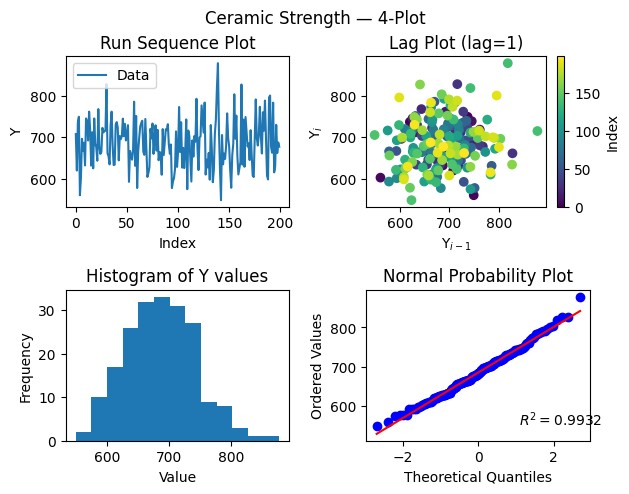
The 4-plot: first stop in any EDA

The NIST handbook recommends starting every univariate EDA with the 4-plot (NIST 1.3.3.5): a 2×2 composite of the run-sequence plot, lag plot, histogram, and normal probability plot. Together these four panels answer the four fundamental questions:

1. Is the process fixed (constant location)?

2. Is the process random (no autocorrelation)?

3. Is the distribution unimodal?

4. Is the distribution approximately normal?

from drippy import four_plot

fig, axes = four_plot(data)
fig.suptitle("Ceramic Strength — 4-Plot", y=1.02)
plt.show()

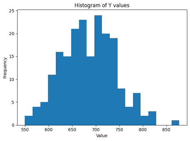
Fluent API

Every plot function is also available as a method on EDAData:

fig, ax = data.histogram(bins=20)
plt.show()

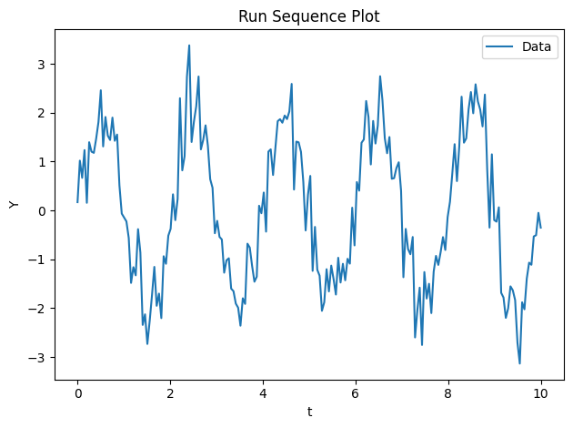
Time-series data

t = np.linspace(0, 10, 200)
noise = rng.normal(scale=0.5, size=200)
y_ts = 2.0 * np.sin(2 * np.pi * 0.5 * t) + noise
data_ts = EDAData(y=y_ts, t=t)

fig, ax = data_ts.run_sequence_plot()
plt.show()

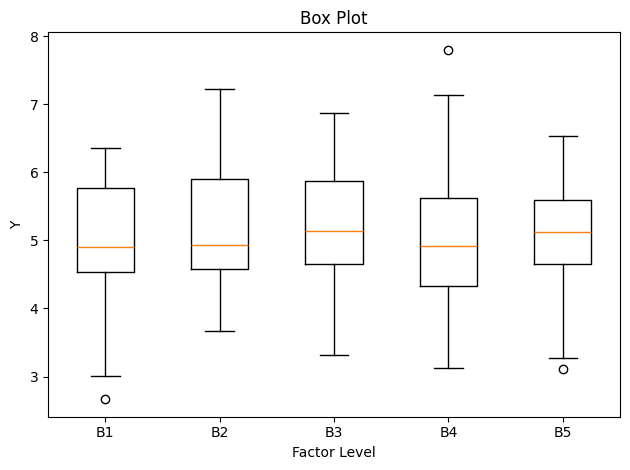
One-factor (categorical) data

batches = ["B1", "B2", "B3", "B4", "B5"]
x_cat = np.repeat(batches, 20)
locs = [5.0, 5.5, 4.8, 5.2, 5.1]
y_cat = np.concatenate([rng.normal(loc=l, scale=1.0, size=20) for l in locs])
data_cat = EDAData(y=y_cat, x=x_cat)

fig, ax = data_cat.box_plot()
plt.show()

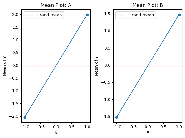
Multi-factor / DOE data

A = np.tile([-1, 1], 8)
B = np.repeat([-1, 1], 8)
y_doe = 2.0 * A + 1.5 * B + rng.normal(scale=0.3, size=16)
data_doe = EDAData(y=y_doe, factors={"A": A, "B": B})

fig, axes = data_doe.doe_mean_plot()
plt.show()