Univariate Plots

Univariate EDA assumes the model y = c + e — a fixed location c plus random error e. The goal is to characterise the distribution of e and check whether the data are truly random and stationary.

Reference: NIST Handbook Chapter 1.3.3

%matplotlib inline
import numpy as np
import matplotlib.pyplot as plt
from drippy import EDAData
from drippy import (
    run_sequence_plot,
    lag_plot,
    histogram,
    normal_probability_plot,
    four_plot,
    ppcc_plot,
    weibull_plot,
    probability_plot,
    box_cox_normality_plot,
    bootstrap_plot,
    box_cox_linearity_plot,
)

rng = np.random.default_rng(42)

# Normal data — 200 ceramic-strength-like measurements
y = rng.normal(loc=688.0, scale=65.0, size=200)
data = EDAData(y=y)

# Positive-only data — component lifetimes following a Weibull distribution
y_pos = rng.weibull(2.0, size=100) * 500
data_pos = EDAData(y=y_pos)

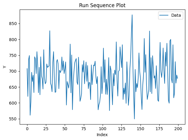
Run Sequence Plot (NIST 1.3.3.25)

Plots y in the order the measurements were taken. Drifts, shifts, or periodic patterns visible here indicate the data are not stationary.

fig, ax = run_sequence_plot(data)
plt.show()

Supply a physical time axis via t:

t = np.linspace(0, 10, 200)
data_t = EDAData(y=y, t=t)
fig, ax = run_sequence_plot(data_t)
plt.show()

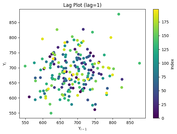
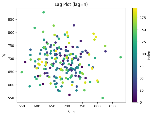
Lag Plot (NIST 1.3.3.15)

Scatters y[i] against y[i − lag]. A structureless cloud confirms randomness; patterns (lines, ellipses) reveal autocorrelation.

fig, ax = lag_plot(data)
plt.show()

fig, ax = lag_plot(data, lag=4)
plt.show()

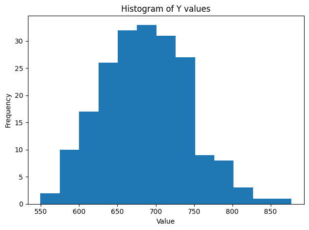
Histogram (NIST 1.3.3.14)

Shows the frequency distribution of y. Look for symmetry, outliers, and whether the shape matches a known family.

fig, ax = histogram(data)
plt.show()

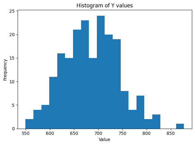
fig, ax = histogram(data, bins=20)
plt.show()

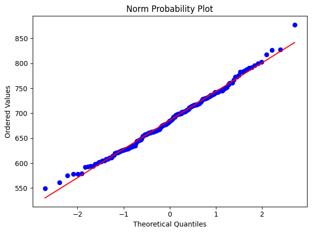
Normal Probability Plot (NIST 1.3.3.21)

Ordered data against normal quantiles. A straight line indicates normality; curvature suggests skew or heavy tails.

fig, ax, _ = normal_probability_plot(data)
plt.show()

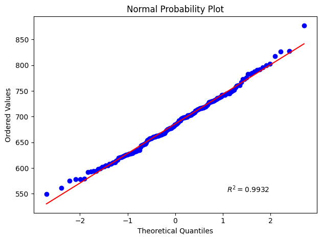
fig, ax, rsq = normal_probability_plot(data, return_rsquared=True)
print(f"R² = {rsq:.4f}")
plt.show()

R² = 0.9932

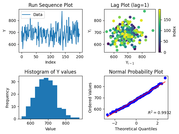
4-Plot (NIST 1.3.3.5)

The 4-plot combines the run-sequence plot, lag plot, histogram, and normal probability plot in a single 2×2 figure — the recommended first step for any univariate EDA.

fig, axes = four_plot(data)
plt.show()

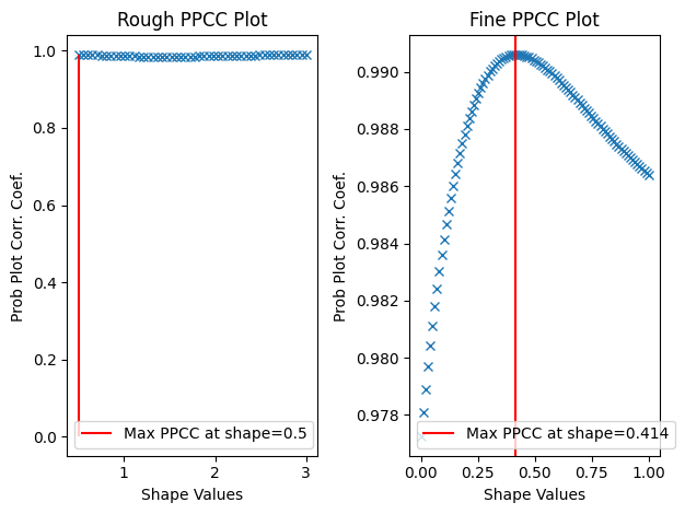
PPCC Plot (NIST 1.3.3.6)

The Probability Plot Correlation Coefficient (PPCC) plot finds the shape parameter of a distribution family that best fits the data. The rough panel locates the maximum; the fine panel zooms in.

fig, axes = ppcc_plot(data_pos)
plt.show()

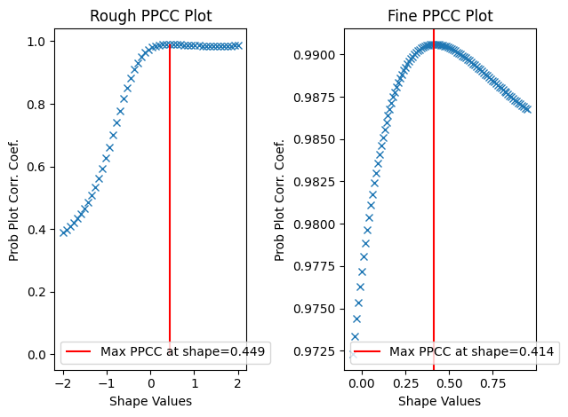
fig, axes = ppcc_plot(data_pos, rough_range=(0.5, 3.0))
plt.show()

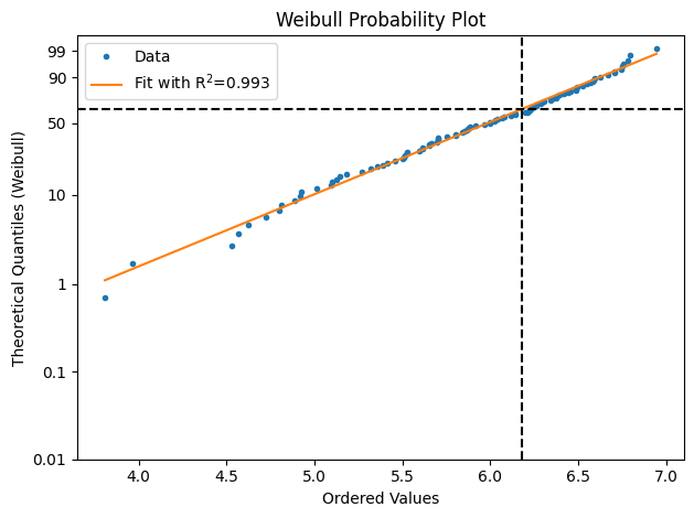
Weibull Plot (NIST 1.3.3.30)

Linearised Weibull probability plot for positive failure-time or strength data. The fitted slope is the Weibull shape parameter β; the vertical dashed line marks the characteristic life η.

fig, ax = weibull_plot(data_pos)
plt.show()

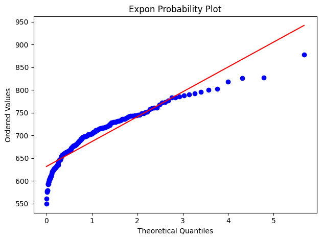
Probability Plot (NIST 1.3.3.24)

Generalisation of the normal probability plot: compare ordered data against the quantiles of any scipy.stats distribution.

fig, ax = probability_plot(data)
plt.show()

fig, ax = probability_plot(data, distribution="expon")
plt.show()

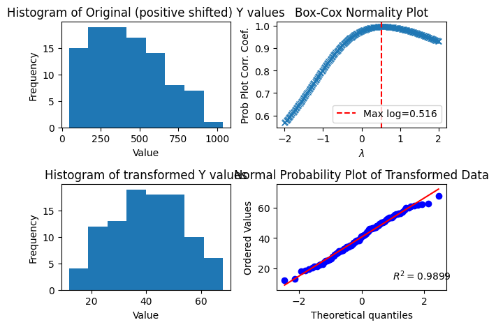
Box-Cox Normality Plot (NIST 1.3.3.8)

Finds the Box-Cox power λ that maximises normality of positive data. The 2×2 grid shows the original histogram, the PPCC-vs-λ curve, the transformed histogram, and the normal probability plot of the transformed data.

fig, axes = box_cox_normality_plot(data_pos)
plt.show()

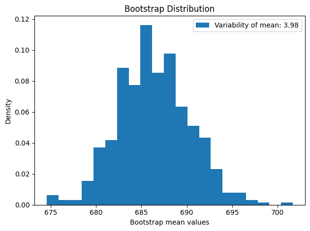
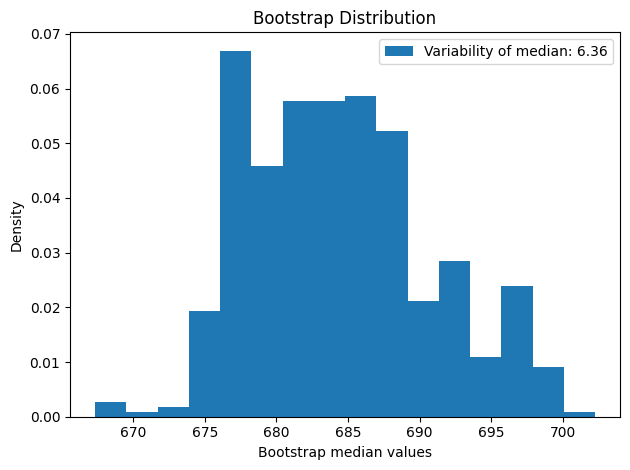
Bootstrap Plot (NIST 1.3.3.4)

Resamples the data to approximate the sampling distribution of any statistic. The histogram of the bootstrap distribution gives a non-parametric confidence interval for the statistic.

fig, ax = bootstrap_plot(data, n_bootstrap=500)
plt.show()

fig, ax = bootstrap_plot(data, statistic=np.median, n_bootstrap=500)
plt.show()

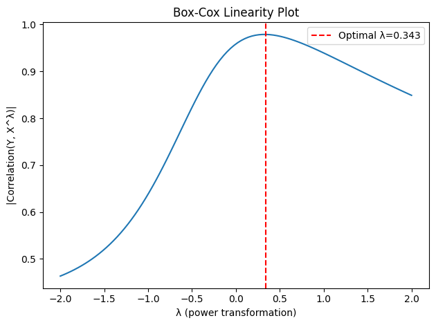
Box-Cox Linearity Plot (NIST 1.3.3.9)

Plots |corr(y, x^λ)| across a range of λ values to identify the power transformation of x that best linearises the relationship with y. Requires x > 0.

x_pos = np.linspace(0.1, 10.0, 50)
y_lin = 3.0 * x_pos**0.5 + rng.normal(scale=0.5, size=50)
data_lin = EDAData(y=y_lin, x=x_pos)

fig, ax = box_cox_linearity_plot(data_lin)
plt.show()