Multi-Factor / DOE Plots

Multi-factor EDA analyses designed experiments (DOE) where multiple factors are varied simultaneously. Pass named factor arrays via the factors dict to EDAData.

The plots answer: which factors drive location or spread, and what does the response surface look like?

Reference: NIST Handbook Chapter 5

%matplotlib inline
import numpy as np
import matplotlib.pyplot as plt
from drippy import EDAData
from drippy import (
    doe_scatter_plot,
    doe_mean_plot,
    doe_sd_plot,
    contour_plot,
)

rng = np.random.default_rng(42)

# 2-factor full-factorial DOE — 16 runs
# Factor A: temperature (+1 = high, −1 = low)
# Factor B: pressure (+1 = high, −1 = low)
# Response: process yield
A = np.tile([-1, 1], 8)
B = np.repeat([-1, 1], 8)
y = 2.0 * A + 1.5 * B + 0.5 * A * B + rng.normal(scale=0.3, size=16)
data = EDAData(y=y, factors={"Temperature": A, "Pressure": B})

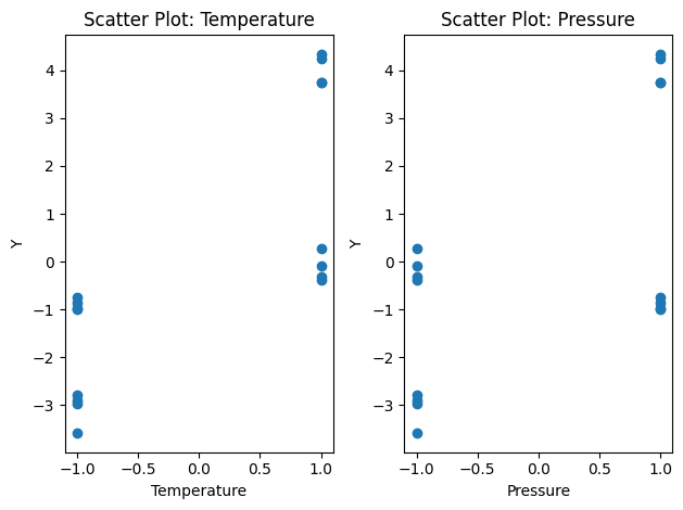
DOE Scatter Plot

One subplot per factor. Scatters y against each factor’s coded level to reveal the raw relationship before any modelling.

fig, axes = doe_scatter_plot(data)
plt.show()

DOE Mean Plot

For each factor, plots the mean response at each level and draws the grand mean as a reference. Steep slopes signal large main effects.

fig, axes = doe_mean_plot(data)
plt.show()

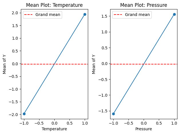
Temperature has a larger slope than Pressure, indicating a stronger effect on yield.

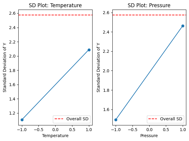
DOE SD Plot

Like the mean plot but for within-level standard deviations. Detects factors that affect process variability, not just location.

fig, axes = doe_sd_plot(data)
plt.show()

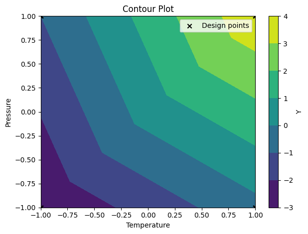
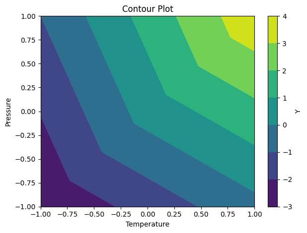
Contour Plot (NIST 1.3.3.10)

Interpolates a contour surface over the 2-factor design space. Requires exactly two factors. Optimal conditions appear as peaks or ridges in the surface.

fig, ax = contour_plot(data)
plt.show()

Overlay the actual design points:

fig, ax = contour_plot(data, doe=True)
plt.show()